Maintaining open-source software usually involves juggling many possible improvements with only so much time to work on them.

FastTrack, the open-source tool I started for tracking multiple deformable objects in videos during my PhD thesis, is no different. The project has grown over the years, but improving performance is especially tough. Finding bottlenecks is just the first step, and every possible optimization needs to be implemented, tested, benchmarked, reviewed, and then either kept or dropped.

Many potential improvements are therefore difficult to justify. An optimization may sound promising but ultimately produce little measurable benefit. Investigating it manually can consume several hours or days, with no guarantee that the resulting code will be faster.

For the development of FastTrack 6.6.0, I decided to test a different workflow: use AI coding tools to accelerate the implementation and evaluation of potential optimization paths, while relying on profiling, automated tests, reproducible benchmarks, and manual code review to retain control over the final result.

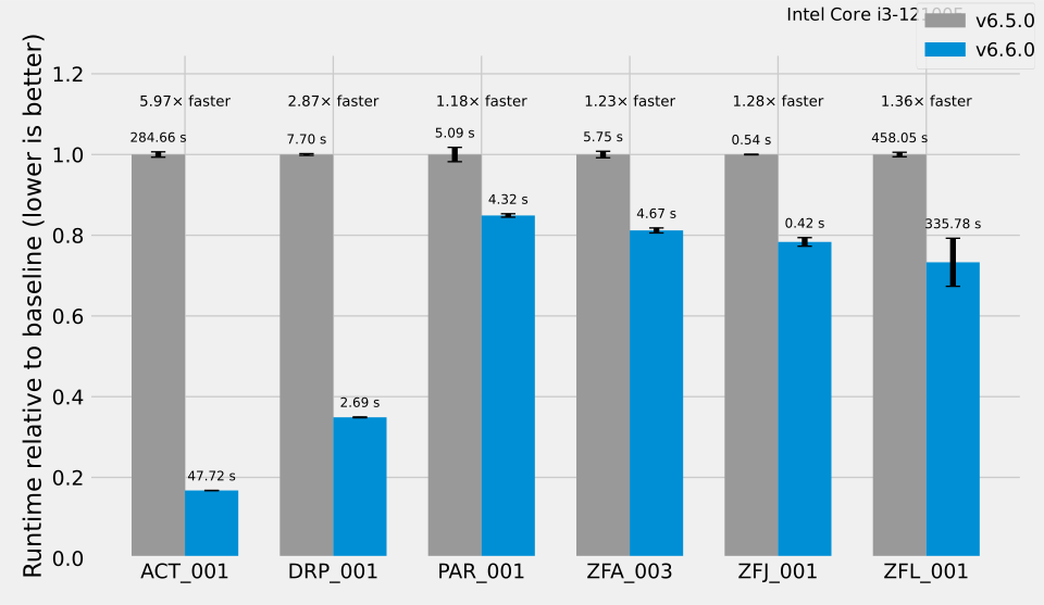
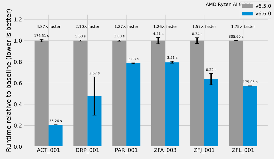
The results were impressive. Every dataset in the benchmark suite ran faster on both systems I tested. Depending on the workload and processor, speedups ranged from about 1.2× to 6×. Overall, the total benchmark time dropped by 48% on an Intel Core i3-12100F and by 56% on an AMD Ryzen AI 9 365, which means overall speedups of 1.93× and 2.25×.

This experiment also taught me something important: the main value of AI here wasn’t in writing software on its own, but in making it much cheaper to try out new ideas.

About FastTrack​

FastTrack is a free, open-source desktop application for tracking multiple objects in video recordings. It combines automatic object detection and identity-preserving tracking with tools for manual review and correction. You can use it on Linux, macOS, and Windows, and its tracking core can be integrated into other C++ and Qt apps through a public API.

The software was first built for scientific work, especially experiments with multiple animals or other deformable objects. In these cases, processing time is important for several reasons:

• Recordings may contain many thousands of frames.
• Multiple recordings may need to be processed as a batch.
• Tracking parameters are often adjusted iteratively.
• Real-time tracking should be performed.

So, even a moderate speedup can save much more time than just one run. Faster processing shortens the whole cycle of picking parameters, tracking, checking results, making corrections, and doing the final analysis.

The maintenance constraint​

FastTrack isn’t a new prototype. It’s a well-established project. It already works, has users, and reflects years of design choices.

When you’re building a new algorithm, big changes to the structure are often fine. But in a mature application, every change has to keep things working the same way across different platforms and real datasets. A faster version isn’t helpful if it causes numerical errors, data races, platform-specific bugs, database issues, or subtle changes in how objects are identified.

Performance work also competes with other development priorities:

• Compatibility with new operating systems.
• Packaging and distribution.
• Bug fixes.
• Feature requests.
• Dependency upgrades.
• Continuous-integration maintenance.

As the main maintainer, I can’t look into every possible optimization myself. Before this experiment, I knew some parts of the tracking pipeline were likely slow, but rewriting each one would have taken more time than I could justify without proof that it would really help.

Why FastTrack was a suitable candidate for AI-assisted optimization​

FastTrack already had two essential components:

1. An automated test suite.
2. A benchmark and accuracy-testing workflow based on representative datasets.

The tests helped catch any behavior changes after each update. The benchmark suite checked whether the modification was faster across several heterogeneous datasets.

A code change might pass all the tests but still slow down the app. Or it might look great in benchmarks but quietly change the tracking results.

Because this infrastructure was already in place, FastTrack was a good fit for trying out AI-assisted development. I didn’t have to trust AI-generated patches just by looking at them. I could compile, test, benchmark, inspect, tweak, or reject them based on real evidence.

The working hypothesis​

The experiment started with a pretty simple idea:

AI coding tools could reduce the implementation cost of testing optimization ideas, including ideas whose benefits were too uncertain to justify implementing manually.

The goal wasn’t to just tell an AI to “make FastTrack twice as fast” and accept whatever it gave me.

Instead, the process was more like supervised performance engineering:

1. Identify or profile an expensive part of the program.
2. Define the expected behavior and relevant constraints.
3. Ask the AI system to analyze or rewrite a bounded section.
4. Inspect the proposed implementation.
5. Compile it with the project’s normal warning and quality settings.
6. Run the functional and accuracy tests.
7. Benchmark the change.
8. Refine it manually or with additional AI iterations.
9. Reject it if the improvement was absent, too small, or obtained at an unacceptable complexity cost.
10. Approve and commit only the final reviewed version.

AI generated most of the first versions. I guided the process, reviewed the code, fixed and simplified things as needed, checked how it worked and performed, and took full responsibility for every change that was committed.

Profiling before optimization​

When optimizing performance, it’s best to start by measuring, not just guessing. The first step was therefore to inspect the tracking pipeline and identify operations that were likely to dominate execution time or scale poorly with the number of objects, pixels, or frames.

Replacing the object-assignment implementation​

One of the most substantial algorithmic changes concerned FastTrack’s implementation of the Hungarian assignment algorithm.

Object tracking requires associating objects detected in the current frame with objects identified in previous frames. FastTrack constructs a cost matrix describing the plausibility of each possible association and solves the resulting assignment problem.

The previous implementation (the best I found five years ago; I benchmarked many available implementations at the time) repeatedly scanned or copied complete matrices and created large temporary allocations. The replacement uses a shortest-augmenting-path formulation with contiguous row-major storage. It also handles square, wide, tall, and empty matrices, avoids physically transposing tall matrices, removes repeated large temporary allocations, and validates malformed input matrices.

This shows why changing the algorithm itself can matter more than just tweaking small parts. Better memory layout and less repeated matrix work can improve both speed and how well the code uses the computer’s cache.

However, this was also one of the areas where validation was most important. Assignment code influences object identities directly. A faster implementation would not be acceptable if it changed assignments unexpectedly or mishandled rectangular or degenerate matrices.

Avoiding unnecessary image rotations​

Another important change removed part of the image-processing work previously used to determine object orientation.

The earlier implementation physically rotated an image region so that an object’s main axis became horizontal. It then divided the rotated image into two regions and calculated properties used to distinguish the head and tail.

The new implementation derives the required information from projected pixel coordinates and statistical moments without first constructing a rotated image. This optimization is interesting because it skips a costly image transformation and instead calculates the needed information directly.

This kind of reformulation is a particularly useful target for AI-assisted exploration. The transformation is mathematically bounded, but implementing it correctly involves enough indexing, coordinate conversion, and statistical calculation that trying it manually may not have been an attractive use of limited maintenance time.

Improving database writes​

Tracking does not end with image analysis. Results must also be stored. The optimization work included changes to the database-insertion path, reducing repeated query setup and reorganizing how values are bound and written within the existing transaction flow.

It’s easy to miss database overhead when profiling a computer vision app. You might assume most of the time goes to image processing, but in reality, repeated setup, allocation, conversion, and insertion inside a frame-by-frame loop can add up.

Reducing repeated work in object selection​

A smaller optimization simplified the object-selection logic used during tracking. Although the corresponding patch changed only a few lines, operations inside a nested frame-and-object loop can accumulate substantial cost over an entire recording.

This is another plus of using AI in the workflow: it makes it easier to try out even small improvements.

As a maintainer, I might skip spending an hour rewriting and testing a few lines if I don’t know the impact. But if a patch can be generated quickly and tested automatically, even small ideas are worth trying.

Balancing parallelism across heterogeneous workloads​

The latest changes add parallel processing to key parts of the tracking pipeline, such as contour processing and cost-matrix calculations. However, parallelism is only used when it actually speeds things up. For smaller workloads, the overhead of managing threads can outweigh the benefits, so the code runs sequentially unless the workload is large enough to justify parallel execution. Thresholds for switching between sequential and parallel processing were set based on benchmarking, not fixed values.

FastTrack handles many kinds of datasets, some with a few large objects, others with many small ones, or complex combinations. Each type stresses different parts of the pipeline. For example, large objects require more image processing, while many small objects make assignment problems bigger. Because of this variety, indiscriminate parallelism can actually slow things down for some cases.

To address this, the implementation uses conditional parallelism: only workloads above a certain size are parallelized, and the best threshold or scheduling strategy can vary depending on the data. AI assistance made it much faster to try, test, and refine these parameters. Instead of finding a single "best" setup, the process focused on quickly evaluating different options to find what works well across a range of real datasets.

As a result, the overall speedup varies by workload and processor, since each dataset stresses a different mix of tasks. The main goal was robust performance for many scenarios, not just maximizing one benchmark.

Changes that were not retained​

Not every proposed optimization was useful. Some changes failed to improve performance, made one dataset faster but another slower, altered output values, added too much complexity, duplicated existing library functions, created unsafe parallel access, increased memory use, relied on invalid assumptions, or passed tests while failing broader accuracy checks. One of the main benefits was being able to discard these failed experiments quickly and at low cost. The AI system was valuable not just for generating patches that worked, but also for making it affordable to test and rule out ideas that were not worth pursuing.

Interpreting the results​

The benchmark results show that the optimizations improve performance across every tested dataset, but the magnitude of the gain varies substantially between workloads and processors. This variation is expected because each dataset stresses a different combination of image processing, contour analysis, cost-matrix construction, object assignment, database access, and parallel execution. Datasets with many objects can benefit more from improvements to assignment and pairwise-cost calculations, while datasets containing fewer but larger or more complex objects may remain dominated by image-level operations. Hardware characteristics also influence the results: the 20-thread Ryzen AI 9 365 provides more opportunities for parallel execution, whereas the 8-thread Intel Core i3-12100F places a lower ceiling on parallel throughput. Nevertheless, the optimized version completed the full benchmark suite approximately 1.93× faster on the Intel system and 2.25× faster on the AMD system, reducing cumulative runtime by about 48% and 56%, respectively. The individual speedups ranged from approximately 1.2× to 6×, demonstrating that the improvements are broadly effective while remaining strongly dependent on workload composition. The appropriate conclusion is therefore not that FastTrack is uniformly six times faster, but that it now completes a diverse set of representative tracking workloads in roughly half the previous time.

What AI implemented and what remained human work​

It is worth being transparent about the division of work.

AI tools generated most of the initial implementation for the optimization patches. This included algorithmic rewrites, local simplifications, candidate parallelizations, and associated test changes.

My work included:

• Identifying the performance objective.
• Directing the profiling and optimization process.
• Deciding which parts of the code could be changed safely.
• Providing constraints and feedback.
• Reviewing generated code.
• Independently running and interpreting tests.
• Rejecting unsuitable approaches.
• Evaluating maintainability.
• Approving and committing the final code.
• Retaining responsibility for the released behavior.

AI as a tool for reducing experimental cost​

The most useful effect of the workflow was economic rather than magical.

Before AI-assisted implementation, each optimization idea had an implementation cost. Even a plausible idea could remain unexplored because that cost was too high relative to its uncertain benefit.

The new workflow changed that balance.

A candidate optimization could be generated, compiled, tested, and benchmarked quickly. If it failed, the loss was limited. If it worked, it could be reviewed and refined. This made it reasonable to explore more paths, including those with uncertain returns.

That is a meaningful change for open-source maintenance, where developer attention is often the scarcest resource.

Conclusion​

FastTrack 6.6.0 demonstrates a practical use of AI-assisted software development in an existing open-source scientific application.

Overall, this work shows that AI-assisted development can deliver meaningful improvements in a mature open-source project when it is combined with strong engineering safeguards. The main benefit was not a single optimization or an isolated benchmark result, but the ability to explore, implement, test, and reject performance ideas much more quickly than would otherwise have been practical. Profiling identified where effort should be focused, automated tests protected correctness, heterogeneous benchmarks revealed workload-dependent effects, and manual review ensured that only maintainable changes were retained. The resulting performance gains demonstrate the value of this approach, but the broader lesson is methodological: AI is most effective when it operates inside a disciplined development process rather than replacing one.

The methodological result is more interesting.

AI made it feasible to implement and evaluate optimization paths that would previously have been too expensive or uncertain to investigate with the available maintenance time. Yet the useful outcome depended on infrastructure and oversight that already existed around the generated code:

• profiling identified meaningful targets;
• automated tests guarded behavior;
• benchmark datasets measured real performance;
• accuracy checks evaluated scientific output;
• manual review protected code quality;
• final approval remained human.

The experiment did not show that AI could autonomously optimize a mature application. It showed that, in a well-tested project, AI can make disciplined software experimentation considerably cheaper. That may be one of its most useful roles for open-source maintainers.

Introduction​

In this tutorial, we will see how to train a custom YOLO model and use it with PyFastTrack to track objects.
There are three parts to this tutorial:

• Annotate the dataset.
• Train the model.
• Use the model.

This tutorial will not require GPU; it will use Google Colaboratory to train the model.

Model annotation​

PyFastTrack requires a YOLO detector that performs segmentation, i.e., that can find which pixels belong to the object and which pixels are not.
Training the model is the most tedious task. There are strategies to reduce the tediousness, but we will focus on the basic approach. We will use LabelMe to annotate manually.
The goal is to draw a polygon to delimitate the object (or objects) and assign it to its class. Several exportation formats are possible in LabelMe, and here, we use the default JSON format that we later convert to generate a formatted YOLO dataset.

Train the model​

First, we must convert the dataset to a format compatible with YOLO. We use labelme2yolo tool:

!pip install labelme2yolo
python -m labelme2yolo --json_dir /path/to/labelme_json_dir/ --val_size 0 --test_size 0.15

That produces a dataset with an architecture as follows.

/path/to/labelme_json_dir/
├─ YOLODataset/
├─ dataset.yaml
├─ labels/
│  ├─ train/
│  ├─ test/
├─ images/
│  ├─ train/
│  ├─ test/

For segmentation, each image is associated with a text label file. It contains the class number and the polygon coordinates to create the segmentation mask, one line per object. The coordinates must be normalized between 0 and 1 (x divided by the image width and y divided by the image height).

Training deep learning models without GPU can be time-consuming or even impossible. Alternatives exist by renting a GPU instance from a provider (OVH, AWS, Google, etc.). A more straightforward option to tinker with a small model is Google Colaboratory. Using Google Colaboratory is relatively straightforward. The first step is to upload the dataset folder to your Google Drive. The second step is to create a Colab notebook, set a GPU for processing using Edit>Notebook settings, and choose GPU.

Inside the notebook, we first mount the Google Drive:

import os
from google.colab import drive

drive.mount('/content/drive')
os.chdir('/content/drive/MyDrive/model/')

Then install the dependencies for YOLOv8:

!pip install ultralytics

To train the model, we use the command below (complete documentation can be found here):

from ultralytics import YOLO

model = YOLO('yolov8m-seg.yaml')
model.train(data='YOLODataset/dataset.yaml', batch=8, epochs=200, imgsz=640)

Google Colaboratory enforces a limitation on GPU usage and runtime time. You can circumvent these limitations by training in several steps adding --resume to the training command to continue the training, or by subscribing to a Colaboratory premium. The resulting weights can be downloaded from Google Drive (YOLODataset/runs/segment) and used for inference.

Use the model​

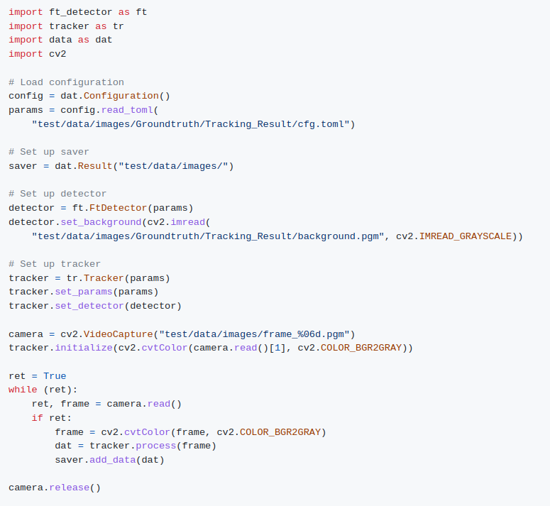
Our custom-trained model can now be used by PyFastTrack to perform the tracking (the tracking can also be done in Google Collab if you want to leverage PyFastTrack GPU capability). The procedure to follow is detailed in the PyFastTrack documentation, and it is straightforward:

• Setup the detector
• Setup the tracker
• Track and save/use tracking data

!pip install pyfasttrack

from pyfasttrack.yolo_detector import YoloDetector
from pyfasttrack.tracker import Tracker
from pyfasttrack.data import Result

import cv2
import os

# Data saver
saver = Result("test/data/images/")

# Set up detector
# See https://github.com/ultralytics/ultralytics/blob/44c7c3514d87a5e05cfb14dba5a3eeb6eb860e70/ultralytics/datasets/coco.yaml for equivalence between coco labels and indexes
yolo_params = {"model": "my_model.pt", "conf": 0.5}
detector = YoloDetector(yolo_params)

# Set up tracker
params = {"spot": 2, "normDist": 1, "normAngle": 2,
          "normArea": 1, "normPerim": 1, "maxDist": 500, "maxTime": 100}
tracker = Tracker()
tracker.set_params(params)
tracker.set_detector(detector)
camera = cv2.VideoCapture(
    "/test/data/images/video.mp4")
dat = tracker.initialize(camera.read()[1])
saver.add_data(dat)
ret = True
while (ret):
    ret, frame = camera.read()
    if ret:
        dat = tracker.process(frame)
        saver.add_data(dat)
camera.release()

PyFastTrack​

Presentation​

PyFastTrack is an open-source Python library that provides the tracking technology of FastTrack in a more modular and customizable way. The parameters and results files are compatible with FastTrack, so analysis performed with PyFastTrack can be reviewed using FastTrack. The library is articulated around two mains class: a base detector and a tracker. The user can implement the base detector and then use it in the tracker to perform the tracking. This modular implementation will facilitate the integration of FastTrack in projects that need more flexibility than the C++ API.

Next week​

The project's current state of development is that the primary foundation blocks are coded. The FastTrack detector and the tracker are implemented and can produce comparable results as FastTrack. For now, PyFastTrack and FastTrack have the same results but with an incertitude of 0.001 pixels and radian on the body ellipse and 0.01 pixels and radian on the head and tail ellipses. However, PyFastTrack is much slower than FastTrack. Supporters can see this week's video update on Kofi for more detail on the first results and a demonstration of the project's current state.

Roadmap​

The project's main focus in the next week will be to optimize PyFastTrack to perform the tracking faster and reach the point of the first public release. In the next few weeks, we will add a deep learning detector (YOLOv8 instance segmentation) so scenes with complex backgrounds can be processed more efficiently, bringing FastTrack into the deep learning era.

Finally, we would like to thank the backers on Kofi: Leonardo Rodriguez-Sosa, and Sushmitha Arumugam, who has supported the development of PyFastTrack. With their contributions, the project can move forward more quickly. Thank you!

What is YOLO​

YOLO (You Only Look Once) is a real-time object detection algorithm using deep learning. It divides the image into a grid. Each cell of this grid is then responsible for detecting objects within itself. YOLO is well known and used because it is relatively fast and accurate. In this proof of concept, we will use YOLOv5, a family of YOLO object detection architecture pre-trained on the COCO dataset.

Why is it interesting for FastTrack​

FastTrack is currently limited to tracking objects in quasi-2-D on very contrasted images with an immobile camera. The software is well adapted for large datasets or datasets with poor quality achieving good accuracy with blazing fast speed. But for users with very detailed datasets, strong 3-D movements, a moving point of view, different types of objects, or complex scenery, FastTrack is limited. Adding a YOLO detector with a pre-or custom-trained model can help these users. They will be able to benefit from a state-of-the-art deep learning detector with the ease and intuitive environment of FastTrack.

Prototype​

To demonstrate the feasibility of using YOLO as a detector for FastTrack, we take a video of running kittens that will first preprocess using YOLOv5 (PyTorch for Python). The resulting video will be tracked using FastTrack GUI.

This video presents quite a challenge to track with 3-D motion, motion blur, occlusions, object deformation, and light kittens on a light background.

The video is processed using YOLOv5x detector pre-trained on the COCO dataset. For each kitten detected, we draw the minimal enclosing image containing the kitten in a white background image. We then repeat the process for all the detected kittens for all the images. This preprocessing simulates what could be done if YOLO was integrated directly inside FastTrack. The direct integration would be much more accurate as each detected object will be processed separately, avoiding object overlap. These images are then tracked using FastTrack, following the standard process.

Implementation​

The implementation of the YOLO detector is relatively straightforward. Currently, the detection is performed using a threshold and then finding the objects in the resulting binary image. The YOLO detection step can be implemented as a class using C++/OpenCV and will return for each image a binary version with the detected objects that will be fed to the FastTrack feature detector. Implementing the YOLO detector will require modifying the GUI by adding a new tab allowing the user to select the specific COCO classes and the detector architecture version. The same modifications will have to be reflected for the CLI with the addition of several command line parameters. Deployment should not cause any problem because the YOLO model files can be deployed with the binary of FastTrack.

Roadmap​

Integrating the YOLO detector inside FastTrack will require some work and testing to have the stability to be made into a stable version for any computer OS. The implementation will be split into several chunks and implemented bit by bit because I have to fit it in between paid contracts, as I can't be on it full time. To speed up the implementation, you can support the project at https://ko-fi.com/bgallois.

The first round of coding for FastAnalyzer is now over. The first alpha version is distributed as a binary for Windows, Linux, and macOS. The public alpha is restricted to 30 minutes of usage, and can be downloaded at https://www.fasttrack.sh/download/Continuous/FastAnalyzer_public_alpha/ with a test dataset. To access the private alpha with unlimited time, behind the scene coding and direct feedback, become a Supporter. In this first cycle, we implemented several essential features that we will detail below.

Project state​

Interface​

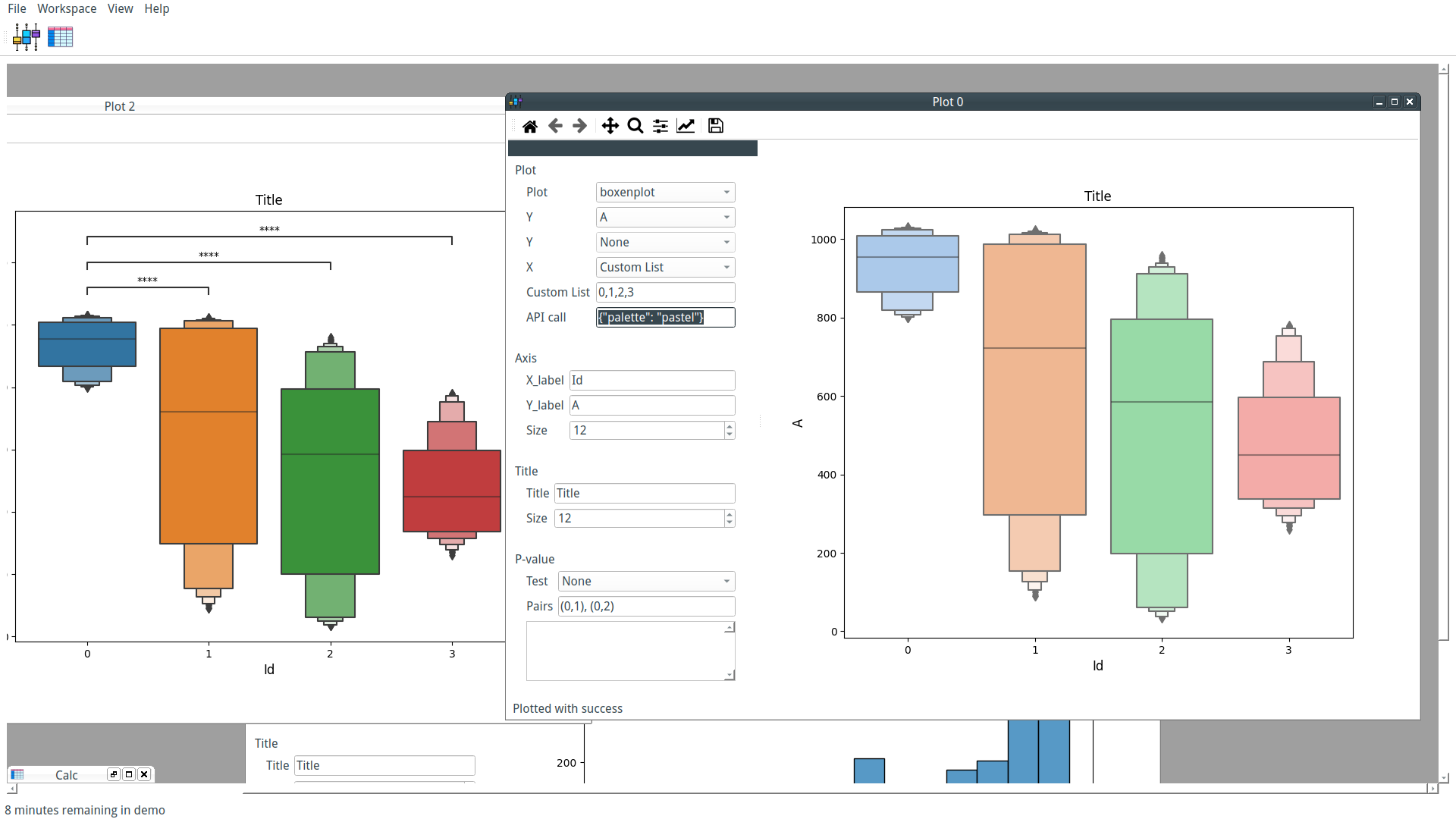
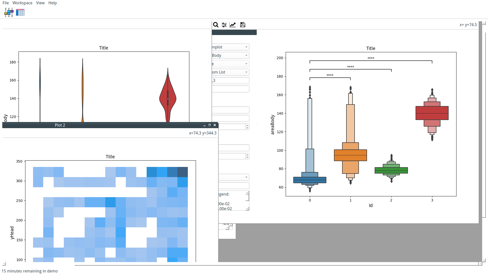
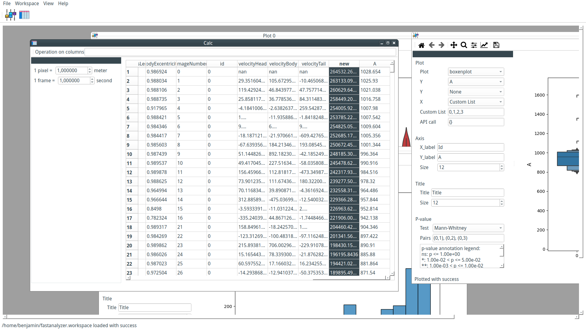
FastAnalyzer interface is an MDI. This interface allows us to see and compare several plots in one glance. That means that each new plot is a unique window inside the interface. Windows can be displayed as tabs or in separate windows (they can be tiled or cascaded). Changes in the data are directly visible in every plot window.

Data loading​

Tracking data from FastTrack (.db and .txt) can be loaded in FastAnalyzer. Once loaded, modified tracking data and plots can be saved as a "workspace" saved and can be reloaded next time. It allows the user to switch seamlessly between several analyses.

Data modification​

Tracking data can be modified using the Calc window. New columns can be created using columns operation. for example, new = xHead**2 will create a new column named new. Regular Pandas operations are supported like sqrt(), diff(), etc. It is also possible to apply a scale to the tracking data to convert pixels and images in meters and seconds.

Data plotting​

Plotting data is the main feature implemented in FastAnalyzer. It supports univariate and bivariate distributions (kdeplot, displot, histplot), and descriptive plot (boxplot, violinplot, boxenplot, swarmplot). Simple features like title, labels, and label size are directly modifiable in the interface. For more advanced users, it is possible to write in the interface a Python dictionary that will be passed in the plot function to call directly advanced features. For example, changing the color palette can be done by writing {"palette": "pastel"} in the lowLevelApi field.

Data statistical significance​

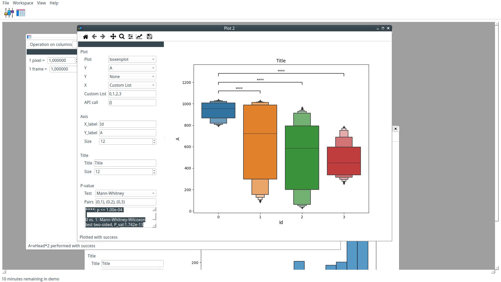
P-values calculation using several standard tests are implemented. Choose the test, write the pair where you want to test, for example, (0,1), (0,2), and FastAnalyzer will directly draw the result on the plot and the detail of the test in the interface.

Conclusion​

The first round of development of FastAnalyzer already offers a software that can produce standard academic plots with statistical significance tests, adjustable titles, and labels. After some first feedback from users, the second round of development will tackle the software performance and robustness with the development of a test suite.

Tracking objects from video recording is generally only the first step of any scientific analysis. The second task, the trajectory analysis, can be quite daunting. Numerous tools are available, from scripting languages to complete user interface environments that require various learning curves.

FastTrack allows an easy and fast tracking from any video recording. To make the trajectory analysis as fast and easy as possible, we started the development of FastAnalyzer. FastAnalyzer is built on top of the Python scientific ecosystem (SciPy, NumPy, Matplotlib and Seaborn) and of the existing FastAnalysis library.

The goal is to integrate the power and versatility of the Python ecosystem in an intuitive user interface tailored to process result file from FastTrack.

The road map to version alpha is as follows:

1. Interface design
2. Basic plot capability
3. Session managment to save and recover plots
4. Master plot theming
5. Statistical analysis

You can see below preview of the software in the current state of development.

As mentioned in previous posts, FastTrack on Windows is slow compared to the Linux and macOS versions. Since version 6.2.5, the tracking speed dramatically improved on Windows.

Problem​

One user reported a bug involving a memory leak on Windows for a specific video format. We investigated this bug and were able to find that it came from the OpenCL library. OpenCL was unable to share a buffer leading to multiple deep copies of images and ultimately a RAM overload. This bug was restricted to the tracking class and reproducible only with a specific video. A hotfix was deployed by deactivating OpenCL.
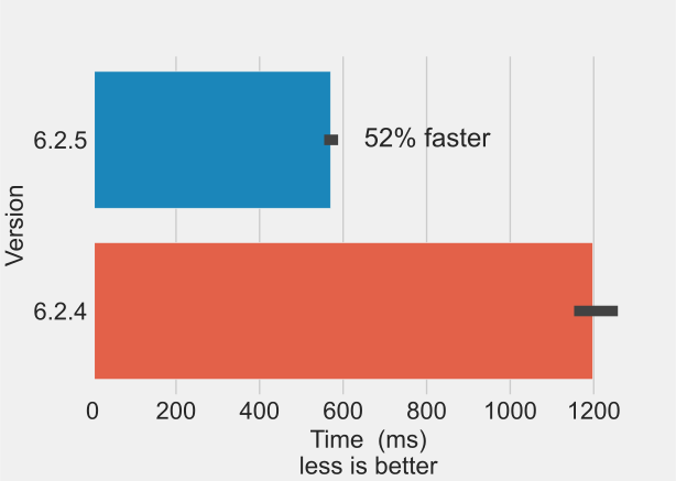
As usual, we run the performance benchmark and no changes were seen... except for Windows (see graph). Surprisingly, deactivating OpenCL increases tracking performance by 52% on Windows.

OpenCL​

"OpenCL (Open Computing Language) is a framework for writing programs that execute across heterogeneous platforms" CPUs, GPUs, DSPs, and FPGAs. OpenCV uses OpenCL by the mean of the transparent API that adds hardware acceleration with a minimal change in the code (use UMat instead of Mat to store images). Using hardware acceleration can increase performance when expensive operations are applied to the image, otherwise, the overhead time to moving the data to the GPU dominate.
There is numerous posts (1,2) on the internet that talk about performance issues with OpenCL. Only one thing is certain, deactivating OpenCL in FastTrack leads to consistent performance across platforms.

In this post, we will use Hyperfine to compare the performance of several versions of FastTrack to see how FastTrack performance has improved or degraded over time.

Methods​

We will automate the benchmark with a python script that will:

1. Select the FastTrack version.
2. Compile FastTrack.
3. Run hyperfine.

  1 import os
  2
  3 def compile(versions, cmd):
  4   for i in versions:
  5     os.system("make distclean -s")
  6     os.system("git checkout -f v{}".format(i))
  7     if i[0] == "6": # Choose qt version
  8       os.system("qmake6 CONFIG+=release src/FastTrack-Cli.pro")
  9     elif i[0] == "5":
 10       os.system("qmake CONFIG+=release src/FastTrack-Cli.pro")
 11     os.system("make")
 12     os.system("make clean")
 13     os.system("mv build_cli {}".format(i))
 14     cmd += "\'{}/fasttrack-cli --path test/dataSet/images/frame_000001.pgm --cfg test/dataSet/images/Groundtruth/Tracking_Result/cfg.toml\' ".format(i)
 14   return cmd
 15
 16 versions = ["6.2.4", "6.2.3", "6.2.1", "6.2.0", "6.1.2", "6.0.0", "5.3.5", "5.2.3"]
 17 cmd = compile(versions, "hyperfine -w 20 -m 100 ")
 18 os.system("git checkout -f master")
 19 os.system(cmd + "--export-markdown benchmark.md")

Results​

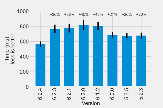
The results of the benchmark are displayed in the graph below with horizontally the version of FastTrack (left is the more recent), and vertically the mean time to perform 50 tracking analyses of the test dataset (less time is better). We can see two interesting breakpoints of performance.

The fastest version is by far the 6.2.4 (latest at the time of writing). This is due to the optimized rewriting of a core function of the tracking. This function computes the object's direction and is used ~nObject*nImage times. A slight gain can greatly impact the overall performance.

We see a degradation of performance between versions 6.0.0 and 6.1.2. This degradation was introduced when FastTrack started to use the SQLite database as a backend. In version 6.0.0 and prior, tracking data were directly saved as a plain text file. This was fine for the tracking but loading the data for reviewing was consuming a lot of RAM and was very slow. Version 6.1.0 and later introduced an SQLite database to store the tracking data but still keep the plain text file for compatibility. This development choice increased performance for the tracking review but slightly degraded the tracking time. Inserting data in the database is faster but generating and writing the text file needed to keep the compatibility introduces a small time overhead degrading the tracking performance. Overall, tracking plus reviewing was faster.

Less significantly, we see a slight increase in performance between versions 6.1.2 and 6.2.3 caused by small optimizations in the code. We see also that migrating from Qt5 (FastTrack 5.3.5 and prior) to Qt6 (FastTrack 5.3.5 and later) doesn't change the performance.

Conclusion​

A tracking analysis is the repetition of a few functions on a lot of images. Marginal gains on these functions can cumulate to a large increase in tracking speed. We work to increase the overall performance with each release of FastTrack and there is still gain to be found.

Since version 6.2.0, FastTrack has been compilated using MinGW_w64 instead of MSVC2019. MinGW_w64 is a fork of the MinGW project that provides the GCC compiler for Windows. With a "better-conforming and faster math support compared to VisualStudio's" and a pthreads library, this compiler yields better performance for the OpenCV library and thus for FastTrack.

Compiling FastTrack using MinGW_w64 provides several improvements. First, it provides the getopt.h header necessary to the FastTrack-Cli. From version 6.2.0, the command line interface of FastTrack is available natively on Windows. Secondly, OpenCV compiled using MinGW_w64 is more performant than with MSVC and Qt seems more responsive. Finally, the bundle (executable plus DLLs) is lighter than its MSVC counterpart (42,7 MB vs 62.8 MB).

Compiling FastTrack using MinGW_w64 comes with some challenges. The main dependency of FastTrack is OpenCV and it does not provide pre-built binaries for MinGW_w64, therefore, we need to compile OpenCV from sources. This compilation is done one time in this GitHub repository and files are downloaded at compile time to save processing energy. Conveniently, Qt provides pre-built binaries and the whole MinGW_w64 toolchains in its archives. Installing Qt and MinWG_w64 can be done very easily without external sources. The windeployqt Qt tool takes care of the DLLs (Qt and MinGW_x64) needed at runtime and the resulting bundle is very light. MinGW_w64 version of Qt does not provide the QtWebEngine, thus, the in software documentation is not available anymore.

To conclude, MinGW_w64 version of FastTrack has better performance, a lighter footprint with only one drawback: recompile OpenCV when newer versions will be available. For developers, the environment is easier to set up with only three commands necessary.

Copyright (C)  FastTrack.
Permission is granted to copy, distribute and/or modify this document. This program is distributed in the hope that it will be useful, but WITHOUT ANY WARRANTY; without even the implied warranty of MERCHANTABILITY or FITNESS FOR A PARTICULAR PURPOSE.

FastTrack performance comparison between Linux and Windows​

FastTrack is a multi-platform application available for Linux, macOS, and Windows. In this post, we will compare the performance of the Linux and Windows versions. We will see that the performance depends a lot on how OpenCV was built and how to build it for performance.

The setup​

The benchmark will be performed using FastTrack version 6.1.1 on a computer with an Intel(R) Core(TM) i7-8565U and 16Go of RAM.
The Linux version was compiled using the GCC compiler with the default release flag of Qt. We used two Windows compilers: MSVC 2019 used for the FastTrack stable release, and MinGW_64 (GCC for Windows. MinGW_64 is not used for binary releases because it lacks the QtWebEngine package but a lighter version of FastTrack can be compiled using the NO_WEB compilation flag). We use OpenCV 4.5.5 and Qt 6.2.2 to perform the benchmark. We chose the test dataset of FastTrack ZFJ_001 with the parameters included with it and the PAR_001 from the two-dimensional dataset.

Results​

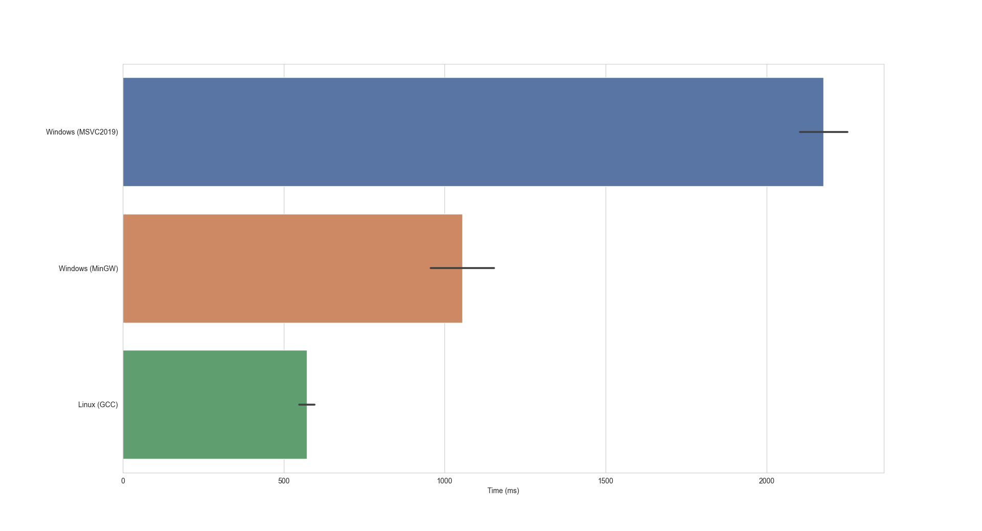
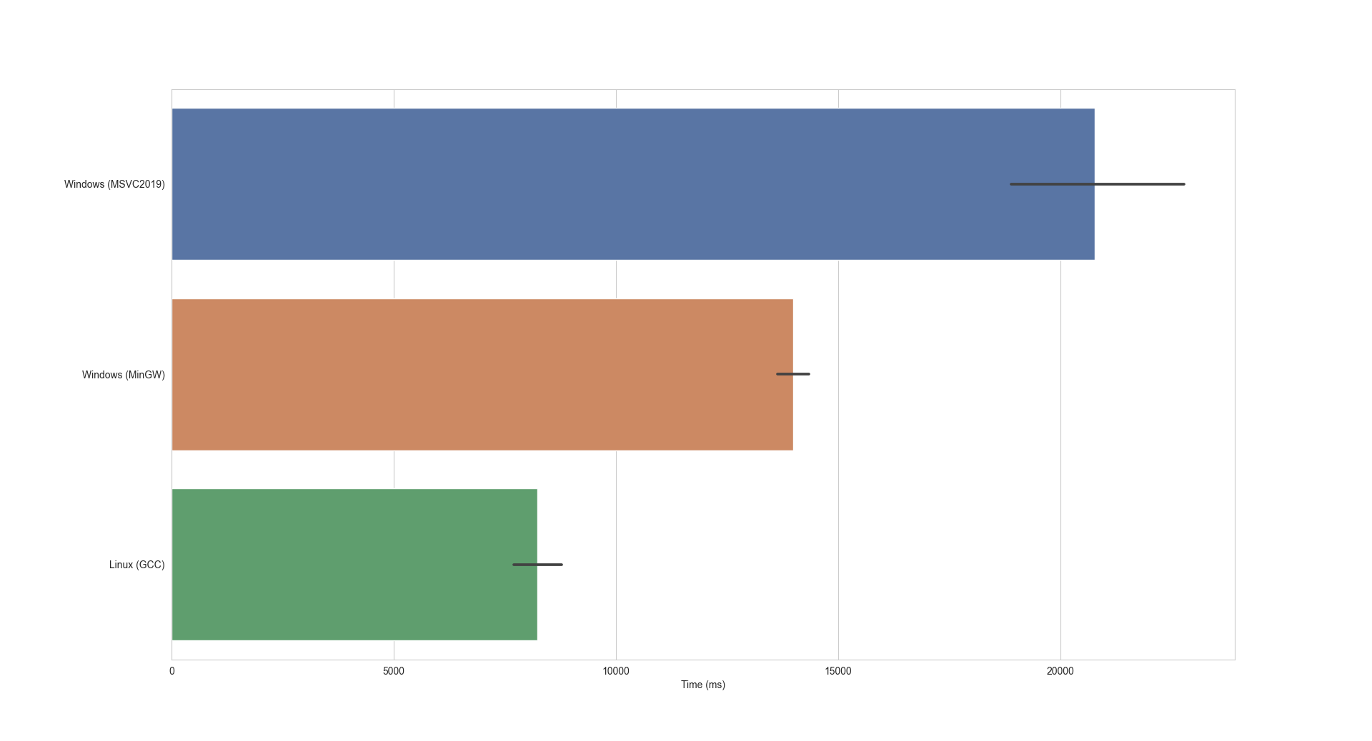
The results of the benchmark are displayed in Figure.1 for ZFJ_001 and Figure.2 for PAR_001. We see that the tracking is significantly slower on Windows than on Linux and that the MinGW_64 compiler yield better performance than MSVC2019.

Figure 1. Benchmark for ZFJ_001.

Figure 2. Benchmark for PAR_001.

These results can be explained by several factors. First, compiler optimizations are not the same and it seems that out-of-the-box Qt and OpenCV are generally faster with GCC. Another point is that FastTrack writes heavily on the disk using both the SQLite database and plain text files. I/O performance varies widely depending on operating system and hardware and is generally better on Linux.

In our case, we can pinpoint a large part of the performance difference to the core operations of the tracking (object detection and ellipse computation) powered by OpenCV that are significantly slower on Windows.

What we can do​

Performance can be improved by tweaking compiler optimization flags and compiling OpenCV using system-specific optimizations if available.

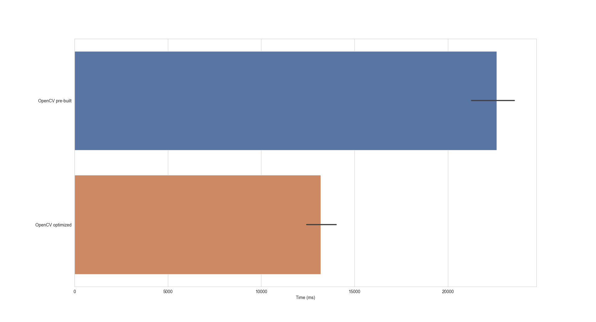
Figure.3 presents the performance for the pre-built OpenCV library and the optimized version compiled with MSVC2019. Optimized OpenCV was compiled with TBB, OpenMP, and IPP enabled and is 1.7 times faster than the pre-built version but still 1.6 times slower than the Linux version.

Figure 3. Pre-built vs omptimized OpenCV library (PAR_001).

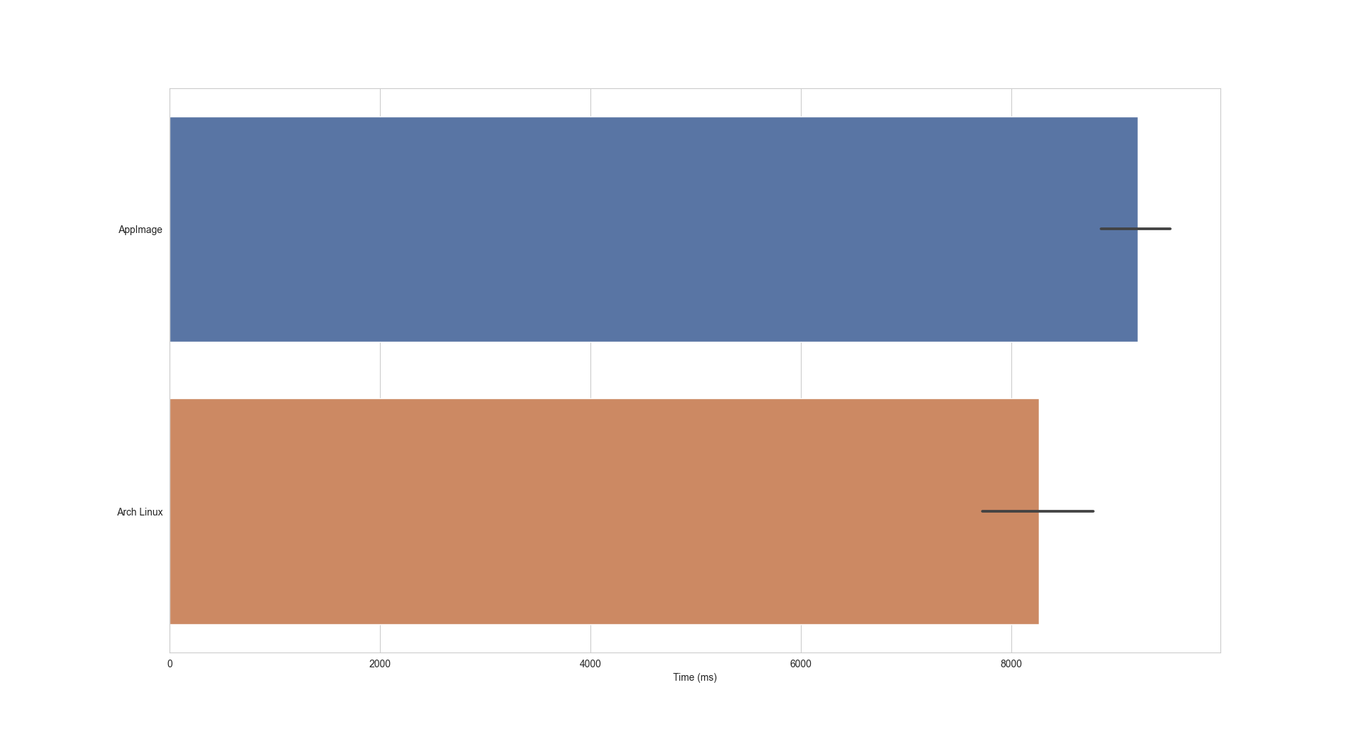
On Linux, OpenCV is compilated as packaged by the Linux distribution. For example, ArchLinux and Ubuntu are not packaged with the same flags enabled and there is still room for performance improvement. In Figure.4, we compare the performance of the AppImage packaged on Ubuntu with the ArchLinux version available on AUR. We see that the native package is slightly faster than the AppImage but still performing very well.

Figure 4. AppImage vs Arch Linux package from AUR (PAR_001).

Final words​

Pre-built binaries of FastTrack will most likely perform better on Linux than on Windows for equivalent hardware. Most Linux distributions will provide a pre-built OpenCV library well optimized whereas FastTrack for Windows is built against the pre-built OpenCV library for MSVC. A custom compilation of OpenCV and FastTrack with platform-specific optimizations will provide maximum performance in any case.
Ultimately, switching to MinGW_64 will be the only way to start to fill the performance gap on Windows. In the next post, we will see how to compile OpenCV and (light) FastTrack with MinGW_64 and if it is possible to have performance as best as the standard Linux version.

Reference​

OpenCV compilation flags